Basic Usage
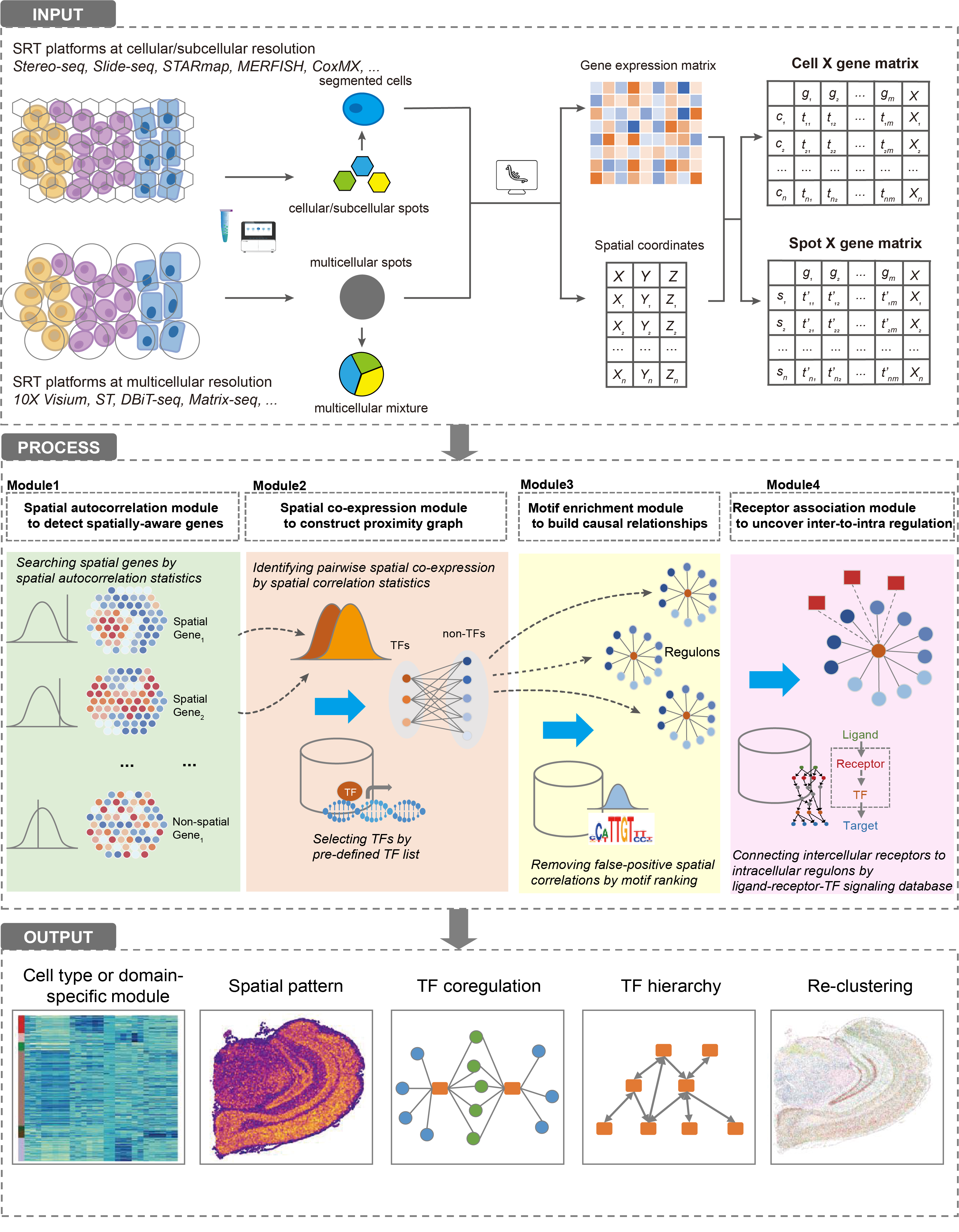
Workflow
Usage
The package provides functions for loading data, preprocessing data, reconstructing gene network, and visualizing the inferred GRNs. The main functions are:
Load and process data
Compute TF-gene similarities
Create modules
Perform motif enrichment and determine regulons
Calculate regulon activity level across cells
Visualize network and other results
Example workflow
from spagrn import InferRegulatoryNetwork as irn

if __name__ == '__main__':  #notice: to avoid concurrent bugs, please do not ignore this line!
        database_fn='mouse.feather'
        motif_anno_fn='mouse.tbl'
        tfs_fn='mouse_TFs.txt'

        # load Ligand-receptor data
        niches = pd.read_csv('niches.csv')

        # Load data
        data = irn.read_file('data.h5ad')

        # Preprocess data
        data = irn.preprocess(data)

        # Initialize gene regulatory network
        grn = irn(data)

        # run main pipeline
        grn.infer(database_fn,
                motif_anno_fn,
                tfs_fn,
                niche_df=niches,
                num_workers=cpu_count(),
                cache=False,
                save_tmp=True,
                c_threshold=0.2,
                layers=None,
                latent_obsm_key='spatial',
                model='danb',
                n_neighbors=30,
                weighted_graph=False,
                cluster_label='celltype',
                method='spg',
                prefix='project',
                noweights=False)
All results will be save in a h5ad file, default file name is spagrn.h5ad.
Visualization
SpaGRN offers a wide range of data visualization methods.
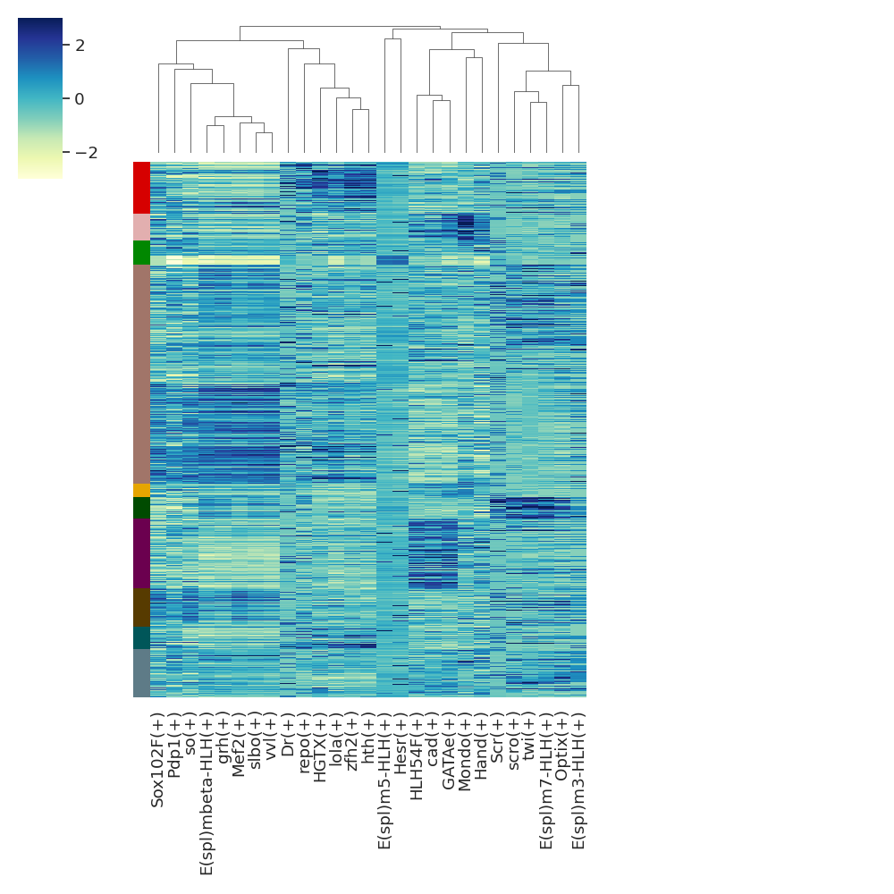
1. Heatmap
read data from previous analysis:
data = irn.read_file('spagrn.h5ad')

auc_mtx = data.obsm['auc_mtx']
plot:
prn.auc_heatmap(data,
        auc_mtx,
        cluster_label='annotation',
        rss_fn='regulon_specificity_scores.txt',
        topn=10,
        subset=False,
        save=True,
        fn='clusters_heatmap_top10.pdf',
        legend_fn="rss_celltype_legend_top10.pdf")
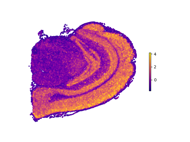
2. Spatial Plots
Plot spatial distribution map of a regulon on a 2D plane:
from spagrn import plot as prn

prn.plot_2d_reg(data, 'spatial', auc_mtx, reg_name='Egr3')
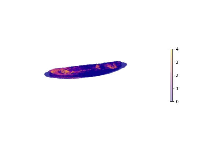
If one wants to display their 3D data in a three-dimensional fashion:
prn.plot_3d_reg(data, 'spatial', auc_mtx, reg_name='grh', vmin=0, vmax=4, alpha=0.3)
Hyperparameters
spatial co-expression methods |
spatial autocorrelation methods |
# nearest neighbor cells (K) |
# SVGs |
# Regulons |
# Target genes |
Detected TF list |
|---|---|---|---|---|---|---|
Ixy |
Intersection of Hx, Ix, Cx, Gx |
5 |
855 |
24 |
497 |
Dlx1, Dlx6, Emx1, Erg, Ets1, Etv4, Fli1, Gbx1, Hivep2, Ikzf1, Klf7, Lhx6, Lhx8,… |
Ixy |
Intersection of Hx, Ix, Cx, Gx |
10 |
978 |
27 |
529 |
Alx4, Dlx1, Dlx6, Emx1, Erg, Ets1, Etv4, Fli1, Gbx1, Hivep2, Ikzf1, Isl1, Klf7,… |
Ixy |
Intersection of Hx, Ix, Cx, Gx |
15 |
1177 |
27 |
529 |
Dlx1, Dlx6, Emx1, Erg, Ets1, Etv4, Fli1, Gbx1, Hivep2, Ikzf1, Klf7, Lhx6, Lhx8,… |
Ixy |
Intersection of Ix, Cx, Gx |
5 |
974 |
23 |
518 |
Dlx1, Dlx6, Emx1, Erg, Ets1, Etv4, Fli1, Gbx1, Hivep2, Ikzf1, Klf7, Lhx6, Lhx8,… |
Ixy |
Intersection of Ix, Cx, Gx |
10 |
1056 |
26 |
575 |
Dlx1, Dlx6, Emx1, Erg, Ets1, Etv4, Fli1, Gbx1, Hivep2, Ikzf1, Klf7, Lhx6, Lhx8,… |
Ixy |
Intersection of Ix, Cx, Gx |
15 |
1286 |
30 |
615 |
Creb3l1, Dlx1, Dlx6, Emx1, Erg, Ets1, Etv4, Fli1, Gbx1, Hivep2, Ikzf1, Klf7,… |
Cxy |
Intersection of Hx, Ix, Cx, Gx |
5 |
856 |
23 |
482 |
Dlx1, Dlx6, Erg, Ets1, Etv4, Fli1, Gbx1, Hivep2, Ikzf1, Klf7, Lhx6, Lhx8, Lmx1a,… |
Cxy |
Intersection of Hx, Ix, Cx, Gx |
10 |
978 |
25 |
536 |
Dlx1, Dlx6, Emx1, Eomes, Erg, Ets1, Etv4, Fli1, Gbx1, Hivep2, Ikzf1, Klf7,Lhx6,… |
Cxy |
Intersection of Hx, Ix, Cx, Gx |
15 |
1177 |
28 |
612 |
Alx4, Dlx1, Dlx6, Emx1, Eomes, Erg, Ets1, Etv4, Fli1, Gbx1, Hivep2, Ikzf1, Klf7,,… |
Cxy |
Intersection of Ix, Cx, Gx |
5 |
974 |
27 |
560 |
Alx4, Dlx1, Dlx6, Eomes, Erg, Ets1, Etv4, Fli1, Gbx1, Hivep2, Ikzf1, Klf7, Lhx6,… |
Cxy |
Intersection of Ix, Cx, Gx |
10 |
1056 |
28 |
585 |
Dlx1, Dlx6, Emx1, Eomes, Erg, Ets1, Etv4, Fli1, Gbx1, Hivep2, Ikzf1, Klf7, Lhx6,… |
Cxy |
Intersection of Ix, Cx, Gx |
15 |
1286 |
31 |
669 |
Alx4, Creb3l1, Dlx1, Dlx6, Emx1, Eomes, Erg, Ets1, Etv4, Fli1, Gbx1, Hivep2,,… |
We have provided a detailed discussion of the three most important hyperparameters and their impact on the results.
The number of nearest neighbor cells (K) used in the Gaussian kernel for capturing local heterogeneity and reducing the influence of high-order neighbors in spatial autocorrelation and co-expression: We evaluated three values for K: 5, 10, and 30. Our observations indicate the following effects: a) Increasing K leads to a larger number of regulons, but without significant differences in their significance. b) The results are relatively stable across different values, although the number of detected regulons increases with increasing K values. c) Considering the biological context, where each cell is typically surrounded by approximately 10 neighboring cells, we have fixed the pipeline to use K =10 as the default value.
The choice of spatial autocorrelation methods: We compared the performance of the intersection gene set using different methods, Hx, Ix, Cx, and Gx. Our analysis revealed the following: a) The majority of the SVGs detected by these methods are shared, indicating a certain level of agreement among the methods. However, each method also uniquely detected some SVGs, suggesting that they may capture different aspects of spatial variation. b) The intersection of all four methods yields more precise regulon boundaries, resulting in a smaller number of regulons and clearer spatial patterns, compared to the intersection of three methods in most cases. Based on these findings, we have chosen to use the intersection of all four methods in our fixed pipeline.
The choice of spatial co-expression methods: We compared the results obtained using two co-expression methods: bivariate Moran’s I Ixy and bivariate Geary’s C Cxy. Our analysis demonstrated the following: The differences in the output results between Moran’s I and Geary’s C are minimal. Specifically, the number of regulons, the TFs identified in the regulons, and the composition of target genes within regulons with the same TF are all similar. Based on these findings, we default to the Morlan’s I method for co-expression network inference in our fixed pipeline.
Warning
Note that it is recommended to utilize the intersection set of spatially specific genes generated by five different gene autocorrelation detection algorithms by default. The intersection strategy ensures a more robust and reliable identification of spatially specific genes. Throughout the manuscript, we have consistently employed the intersection of gene sets unless explicitly stated otherwise.
To mitigate the potential overshadowing effect of large-sample cell types or functional regions on those with a small number of spots or cells, we strongly recommend adopting Moran’s I co-expression method as the default approach, especially for complex organ and tissue structures. This method has proven to be effective in generating spatial GRNs specifically expressed in rare cell types or regions using various datasets. Additionally, users have the option to crop the area of interest, which can increase the sample size of cell types or functional regions with limited spots or cells. This approach has the potential to improve the ranking of specific co-expressed targets, further enhancing the accuracy of the analysis.